Example 01: Conv 1D
Definition
This section will introduce the first concrete example of a numerical solver, which solves an 1D convection problem with constant convection velocity. The governing equation of the problem is:
It is well known that the solution to this problem is:
We integrate the system with zero boundary conditions and a square wave initial condition:
Numerical method
We test two numerical schemes here different in their spatial discretization schemes. The first is a simple first order upwind scheme, i.e.:
This scheme is robust yet highly dissipative. The other scheme we use here is the 5th order WENO scheme proposed by Jiang & Peng 2000. This scheme is 5th order at smooth area and degenerates to 3rd order ENO scheme at the discontinuity. We omit the details of the WENO scheme here and you may find them in the original paper.
Implementation
The implementation for the current example can be found in examples/CONV1D/CONV1D.cpp.
The first step is to build & initialize the mesh & field we used for calculation.
We first define a uniform 1D mesh on the interval \([0, 1]\) with 100 intervals:
auto mesh = MeshBuilder<Mesh>().newMesh(101).setMeshOfDim(0, 0., 1.).build();
Then we define a field u on our mesh and initialize it:
auto u = ExprBuilder<Field>()
             .setMesh(mesh)
             .setName("u")
             .setBC(0, DimPos::start, BCType::Dirc, 0.)
             .setBC(0, DimPos::end, BCType::Dirc, 0.)
             .setLoc(LocOnMesh::Corner)
             .build();

u.initBy([](auto&& i) { return 0.2 <= i[0] && i[0] <= 0.4 ? 1.0 : 0.0; });
We then define the time step dt and convection velocity c
const Real dt = 0.5e-2;
const Real c = 1.0;
and the output stream for results
Utils::TecplotASCIIStream uf("u.tec");
Now we have done all the preparation works. We then start the main loop
for (auto i = 0; i < 100; ++i) {
    // the main body
}
For each time step, we make the following update
By introducing the aforementioned schemes for the spatial derivative, we get the fulling discretized schemes:
// Scheme 1: 1st order upwind scheme
u = u - dt * c * dx<D1FirstOrderBiasedDownwind>(u);
// Scheme 2: 5th order WENO (3rd order at jump) scheme, use 1st order upwind at boundary
u = u - dt * c * d1<DecableOp<D1WENO53Downwind<0>, D1FirstOrderBiasedDownwind<0>>>(u);
We can then run the program and compare the results. Following are animations of the two different cases. We can see that the behavior of the two schemes meet our expectation.
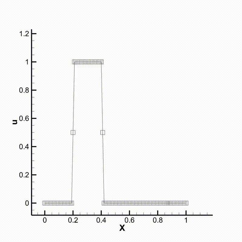
Convection using upwind scheme
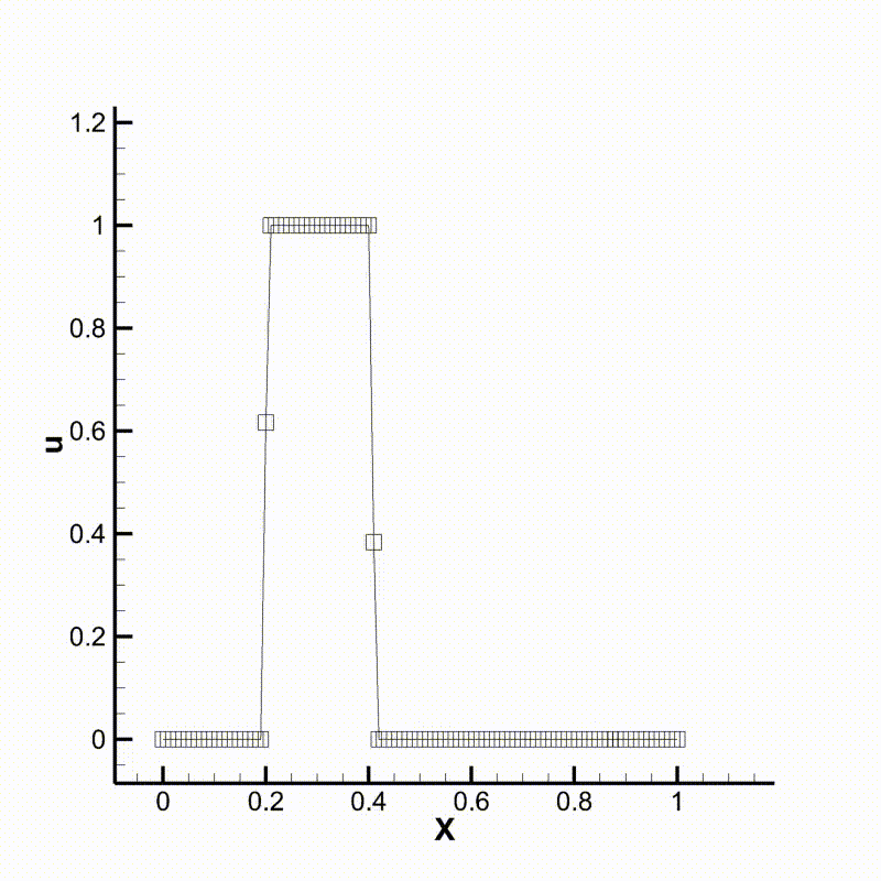
Convection using WENO scheme